Here is an attempt at creating a model that tries to recognize the characters from the famous ‘The Office’ show from their quotes. I am training this model on a dataset containing all the quotes from the show (minus 20% for testing). I then compare various ML and DL models accuracy.
Initialization
Imports
# Basic tools
import re
import nltk
import string
import datasets
import numpy as np
import pandas as pd
import matplotlib.pyplot as plt
from datasets import load_dataset
pd.options.mode.chained_assignment = None  # default='warn'

# Text normalization
from pycontractions import Contractions
from text_normalizer import TextNormalizer
cont = Contractions(api_key="glove-twitter-25")  # 'glove-twitter-100'

# Machine Learning
### Models
from sklearn.naive_bayes import MultinomialNB
from sklearn.tree import DecisionTreeClassifier
from sklearn.linear_model import LogisticRegression, SGDClassifier
from sklearn.ensemble import RandomForestClassifier, ExtraTreesClassifier
### Tools
from sklearn.pipeline import Pipeline
from sklearn.model_selection import train_test_split, cross_val_score
from sklearn.metrics import accuracy_score, confusion_matrix, classification_report
from sklearn.feature_extraction.text import TfidfTransformer, CountVectorizer, TfidfVectorizer

# Deep Learning
import torch
import tensorflow as tf
from tensorflow import keras
from tensorflow.keras import Sequential
from tensorflow.keras import layers, losses, optimizers

# Transformer
from transformers import AutoFeatureExtractor, AutoTokenizer
from transformers import TFAutoModelForImageClassification, TFAutoModelForSequenceClassification
Helper functions
These functions will be helpful in formatting class prediction and showing the evolution of accuracy over DL models.
def predict_class(tf_model, data, class_names):
    """Returns the string model predictions (class name of the largest network output activation)."""

    return np.array(class_names)[tf_model.predict(data).argmax(axis=1)]

def plot_training(history_dict):
    acc = history_dict['accuracy']
    val_acc = history_dict['val_accuracy']
    loss = history_dict['loss']
    val_loss = history_dict['val_loss']

    epochs = range(1, len(loss) + 1)

    plt.figure(figsize=(10, 4))
    plt.subplot(1, 2, 1)
    plt.plot(epochs, loss, 'b--', label='Training')
    plt.plot(epochs, val_loss, 'r-', label='Validation')
    plt.xlabel('Epochs')
    plt.ylabel('Cross-Entropy Loss')
    plt.legend()

    plt.subplot(1, 2, 2)
    plt.plot(epochs, acc, 'b--', label='Training')
    plt.plot(epochs, val_acc, 'r-', label='Validation')
    plt.xlabel('Epochs')
    plt.ylabel('Accuracy')
    plt.legend(loc='lower right')

    plt.show()
Data Import
TheOffice = pd.read_csv('./data/The-Office-Lines-V4.csv', usecols=['season', 'episode', 'title', 'scene', 'speaker', 'line'])
Data Preprocessing
Observation
Here’s the first few lines of the table:
TheOffice.head(5)
| season | episode | title | scene | speaker | line | |
|---|---|---|---|---|---|---|
| 0 | 1 | 1 | Pilot | 1 | Michael | All right Jim. Your quarterlies look very good... |
| 1 | 1 | 1 | Pilot | 1 | Jim | Oh, I told you. I couldn't close it. So... |
| 2 | 1 | 1 | Pilot | 1 | Michael | So you've come to the master for guidance? Is ... |
| 3 | 1 | 1 | Pilot | 1 | Jim | Actually, you called me in here, but yeah. |
| 4 | 1 | 1 | Pilot | 1 | Michael | All right. Well, let me show you how it's done. |
The number of quotes from the top 20 talkative characters:
TheOffice.speaker.value_counts()[0:20]
Michael     10773
Dwight       6752
Jim          6222
Pam          4973
Andy         3698
Kevin        1535
Angela       1534
Erin         1413
Oscar        1336
Ryan         1182
Darryl       1160
Phyllis       962
Kelly         822
Toby          814
Jan           805
Stanley       671
Meredith      556
Holly         555
Nellie        527
Gabe          426
Name: speaker, dtype: int64
n_classes = 10
main_characters = TheOffice['speaker'].value_counts(dropna=False)[:n_classes].index.to_list()
print('Main Characters: ', main_characters)
TheOffice_main = TheOffice.query("`speaker` in @main_characters")
print()
print('Total quotes:                ', len(TheOffice))
print('Quotes from main characters: ', len(TheOffice_main))
Main Characters:  ['Michael', 'Dwight', 'Jim', 'Pam', 'Andy', 'Kevin', 'Angela', 'Erin', 'Oscar', 'Ryan']

Total quotes:                 54626
Quotes from main characters:  39418
Feature engineering
Removing punctuation and lowering the text
punctuation_table = str.maketrans('','',string.punctuation)
TheOffice_main['norm_line'] = TheOffice_main['line'].apply(lambda x: x.translate(punctuation_table))
TheOffice_main['norm_line'] = TheOffice_main['norm_line'].apply(lambda x: x.lower())
TheOffice_main
| season | episode | title | scene | speaker | line | norm_line | |
|---|---|---|---|---|---|---|---|
| 0 | 1 | 1 | Pilot | 1 | Michael | All right Jim. Your quarterlies look very good... | all right jim your quarterlies look very good ... |
| 1 | 1 | 1 | Pilot | 1 | Jim | Oh, I told you. I couldn't close it. So... | oh i told you i couldnt close it so |
| 2 | 1 | 1 | Pilot | 1 | Michael | So you've come to the master for guidance? Is ... | so youve come to the master for guidance is th... |
| 3 | 1 | 1 | Pilot | 1 | Jim | Actually, you called me in here, but yeah. | actually you called me in here but yeah |
| 4 | 1 | 1 | Pilot | 1 | Michael | All right. Well, let me show you how it's done. | all right well let me show you how its done |
| ... | ... | ... | ... | ... | ... | ... | ... |
| 54616 | 9 | 24 | Finale | 8149 | Kevin | No, but maybe the reason... | no but maybe the reason |
| 54617 | 9 | 24 | Finale | 8149 | Oscar | You're not gay. | youre not gay |
| 54619 | 9 | 24 | Finale | 8151 | Erin | How did you do it? How did you capture what it... | how did you do it how did you capture what it ... |
| 54624 | 9 | 24 | Finale | 8156 | Jim | I sold paper at this company for 12 years. My ... | i sold paper at this company for 12 years my j... |
| 54625 | 9 | 24 | Finale | 8157 | Pam | I thought it was weird when you picked us to m... | i thought it was weird when you picked us to m... |
39418 rows × 7 columns
2nd method of normalization by lemmatization, lowering, stopwords and removing punctuation
TheOffice2 = TheOffice.copy()
punctuation_table = str.maketrans('','',string.punctuation)
TheOffice2['norm_line'] = TheOffice2['line'].apply(lambda x: TextNormalizer().normalize_text(text=x, cont=cont)) # 9min to run
TheOffice2['norm_line'] = [' '.join(i) for i in TheOffice2['norm_line']] # because normalize_text() fill table with lists of strings
#TheOffice2['norm_line'] = TheOffice2['line'].apply(lambda x: x.translate(punctuation_table))
#TheOffice_main['norm_line'] = TheOffice_main['norm_line'].apply(lambda x: x.lower())
TheOffice2
| season | episode | title | scene | speaker | line | norm_line | |
|---|---|---|---|---|---|---|---|
| 0 | 1 | 1 | Pilot | 1 | Michael | All right Jim. Your quarterlies look very good... | right jim quarterly look good thing library |
| 1 | 1 | 1 | Pilot | 1 | Jim | Oh, I told you. I couldn't close it. So... | oh told could close |
| 2 | 1 | 1 | Pilot | 1 | Michael | So you've come to the master for guidance? Is ... | come master guidance saying grasshopper |
| 3 | 1 | 1 | Pilot | 1 | Jim | Actually, you called me in here, but yeah. | actually called yeah |
| 4 | 1 | 1 | Pilot | 1 | Michael | All right. Well, let me show you how it's done. | right well let show done |
| ... | ... | ... | ... | ... | ... | ... | ... |
| 54621 | 9 | 24 | Finale | 8153 | Creed | It all seems so very arbitrary. I applied for ... | seems arbitrary applied job company hiring too... |
| 54622 | 9 | 24 | Finale | 8154 | Meredith | I just feel lucky that I got a chance to share... | feel lucky got chance share crummy story anyon... |
| 54623 | 9 | 24 | Finale | 8155 | Phyllis | I'm happy that this was all filmed so I can re... | I happy filmed remember everyone worked paper ... |
| 54624 | 9 | 24 | Finale | 8156 | Jim | I sold paper at this company for 12 years. My ... | sold paper company 12 year job speak client ph... |
| 54625 | 9 | 24 | Finale | 8157 | Pam | I thought it was weird when you picked us to m... | thought weird picked u make documentary alli t... |
54626 rows × 7 columns
Now that the quotes are transformed, we can build some ML and DL models to create character classifiers.
Classification
Variables of interest
y = TheOffice_main['speaker']
y_int = np.array([np.where(np.array(main_characters)==char)[0].item() for char in y])
X = TheOffice_main["norm_line"].to_numpy()
print(y_int)
[0 2 0 ... 7 2 3]
Splitting the dataset
X_train, X_valid, y_train, y_valid = train_test_split(X, y_int, test_size=0.2, random_state=42, shuffle=True)
Logistic Regression
# 9min
logreg = Pipeline([('vect', CountVectorizer()),
                   ('tfidf', TfidfTransformer()),
                   ('clf', LogisticRegression(n_jobs=1, C=1e6, max_iter=10000)),
                  ])

logreg.fit(X_train, y_train)

y_pred_log = logreg.predict(X_valid)

print('accuracy %s' % accuracy_score(y_pred_log, y_valid))
print(classification_report(y_valid, y_pred_log,target_names=main_characters))
accuracy 0.2595129375951294
              precision    recall  f1-score   support

     Michael       0.35      0.44      0.39      2123
      Dwight       0.29      0.26      0.28      1324
         Jim       0.24      0.27      0.26      1274
         Pam       0.20      0.20      0.20       971
        Andy       0.19      0.14      0.16       757
       Kevin       0.12      0.10      0.11       309
      Angela       0.11      0.09      0.10       289
        Erin       0.12      0.09      0.10       301
       Oscar       0.12      0.09      0.10       274
        Ryan       0.10      0.06      0.08       262

    accuracy                           0.26      7884
   macro avg       0.18      0.17      0.18      7884
weighted avg       0.25      0.26      0.25      7884


C:\Users\rened\Anaconda3\lib\site-packages\sklearn\linear_model\_logistic.py:814: ConvergenceWarning: lbfgs failed to converge (status=1):
STOP: TOTAL NO. of ITERATIONS REACHED LIMIT.

Increase the number of iterations (max_iter) or scale the data as shown in:
    https://scikit-learn.org/stable/modules/preprocessing.html
Please also refer to the documentation for alternative solver options:
    https://scikit-learn.org/stable/modules/linear_model.html#logistic-regression
  n_iter_i = _check_optimize_result(
Naive Bayes Classifier
nb = Pipeline([('vect', CountVectorizer()),
               ('tfidf', TfidfTransformer()),
               ('clf', MultinomialNB()),
              ])

nb.fit(X_train, y_train)

y_pred_nb = nb.predict(X_valid)

print('accuracy %s' % accuracy_score(y_pred_nb, y_valid))
print(classification_report(y_valid, y_pred_nb,target_names=main_characters))
accuracy 0.2918569254185693
              precision    recall  f1-score   support

     Michael       0.28      0.98      0.44      2123
      Dwight       0.45      0.11      0.17      1324
         Jim       0.32      0.05      0.08      1274
         Pam       0.41      0.02      0.03       971
        Andy       0.69      0.01      0.03       757
       Kevin       0.00      0.00      0.00       309
      Angela       0.00      0.00      0.00       289
        Erin       0.00      0.00      0.00       301
       Oscar       0.00      0.00      0.00       274
        Ryan       0.00      0.00      0.00       262

    accuracy                           0.29      7884
   macro avg       0.22      0.12      0.08      7884
weighted avg       0.32      0.29      0.17      7884


C:\Users\rened\Anaconda3\lib\site-packages\sklearn\metrics\_classification.py:1318: UndefinedMetricWarning: Precision and F-score are ill-defined and being set to 0.0 in labels with no predicted samples. Use `zero_division` parameter to control this behavior.
  _warn_prf(average, modifier, msg_start, len(result))
Support Vector Machine (SVM)
svm = Pipeline([('vect', CountVectorizer()),
                ('tfidf', TfidfTransformer()),
                ('clf', SGDClassifier(loss='hinge', penalty='l2',alpha=1e-3, random_state=42, max_iter=5, tol=None)),
               ])  # hinge loss == linear SVM
svm.fit(X_train, y_train)

y_pred_svm = svm.predict(X_valid)

print('accuracy %s' % accuracy_score(y_pred_svm, y_valid))
print(classification_report(y_valid, y_pred_svm,target_names=main_characters))
accuracy 0.29921359715880264
              precision    recall  f1-score   support

     Michael       0.37      0.60      0.46      2123
      Dwight       0.31      0.32      0.32      1324
         Jim       0.28      0.16      0.21      1274
         Pam       0.23      0.21      0.22       971
        Andy       0.22      0.19      0.20       757
       Kevin       0.13      0.07      0.09       309
      Angela       0.12      0.09      0.10       289
        Erin       0.19      0.09      0.12       301
       Oscar       0.10      0.04      0.06       274
        Ryan       0.08      0.05      0.06       262

    accuracy                           0.30      7884
   macro avg       0.20      0.18      0.18      7884
weighted avg       0.27      0.30      0.27      7884
Decision Tree Classifier
Tree = Pipeline([('vect', CountVectorizer()),
                 ('tfidf', TfidfTransformer()),
                 ('clf', DecisionTreeClassifier(max_depth=None, min_samples_split=2, random_state=0)),
                ])

Tree.fit(X_train, y_train)

y_pred_Tree = Tree.predict(X_valid)

print('accuracy %s' % accuracy_score(y_pred_tree, y_valid))
print(classification_report(y_valid, y_pred_tree,target_names=main_characters))
accuracy 0.22970573313039067
              precision    recall  f1-score   support

     Michael       0.31      0.42      0.36      2123
      Dwight       0.23      0.26      0.24      1324
         Jim       0.22      0.22      0.22      1274
         Pam       0.18      0.15      0.17       971
        Andy       0.13      0.10      0.11       757
       Kevin       0.07      0.04      0.05       309
      Angela       0.12      0.08      0.09       289
        Erin       0.09      0.05      0.06       301
       Oscar       0.09      0.05      0.06       274
        Ryan       0.06      0.03      0.04       262

    accuracy                           0.23      7884
   macro avg       0.15      0.14      0.14      7884
weighted avg       0.21      0.23      0.22      7884
Random Forest
RanFo = Pipeline([('vect', CountVectorizer()),
                  ('tfidf', TfidfTransformer()),
                  ('clf', RandomForestClassifier(n_estimators=10)),
                 ])

RanFo.fit(X_train, y_train)

y_pred_RanFo = RanFo.predict(X_valid)

print('accuracy %s' % accuracy_score(y_pred_RanFo, y_valid))
print(classification_report(y_valid, y_pred_RanFo,target_names=main_characters))
accuracy 0.2766362252663623
              precision    recall  f1-score   support

     Michael       0.32      0.62      0.42      2123
      Dwight       0.25      0.28      0.26      1324
         Jim       0.24      0.19      0.21      1274
         Pam       0.22      0.15      0.18       971
        Andy       0.18      0.06      0.09       757
       Kevin       0.17      0.04      0.07       309
      Angela       0.12      0.04      0.06       289
        Erin       0.19      0.04      0.06       301
       Oscar       0.12      0.03      0.05       274
        Ryan       0.18      0.02      0.04       262

    accuracy                           0.28      7884
   macro avg       0.20      0.15      0.14      7884
weighted avg       0.24      0.28      0.23      7884
Extremely Randomized Trees
ExtraTree = Pipeline([('vect', CountVectorizer()),
                      ('tfidf', TfidfTransformer()),
                      ('clf', ExtraTreesClassifier(n_estimators=10, max_depth=None, min_samples_split=2, random_state=0)),
                     ])

ExtraTree.fit(X_train, y_train)

y_pred_ET = ExtraTree.predict(X_valid)

print('accuracy %s' % accuracy_score(y_pred_ET, y_valid))
print(classification_report(y_valid, y_pred_ET,target_names=main_characters))
accuracy 0.27638254693049213
              precision    recall  f1-score   support

     Michael       0.32      0.65      0.43      2123
      Dwight       0.25      0.25      0.25      1324
         Jim       0.24      0.19      0.22      1274
         Pam       0.19      0.12      0.15       971
        Andy       0.20      0.07      0.10       757
       Kevin       0.17      0.05      0.07       309
      Angela       0.17      0.04      0.07       289
        Erin       0.15      0.03      0.05       301
       Oscar       0.12      0.03      0.04       274
        Ryan       0.13      0.02      0.03       262

    accuracy                           0.28      7884
   macro avg       0.20      0.14      0.14      7884
weighted avg       0.24      0.28      0.23      7884
data = np.array([[accuracy_score(y_pred_log,y_valid),accuracy_score(y_pred_nb,y_valid),accuracy_score(y_pred_svm,y_valid),accuracy_score(y_pred_Tree,y_valid),accuracy_score(y_pred_RanFo,y_valid),accuracy_score(y_pred_ET,y_valid)]]).round(3)
column_names = ['Logistic Regression','Naive Bayes','SVM','Decision Tree','Random Forest','Extremely Randomzed Trees']
pd.DataFrame(data, index=['Accuracy: '], columns=column_names)
| Logistic Regression | Naive Bayes | SVM | Decision Tree | Random Forest | Extremely Randomzed Trees | |
|---|---|---|---|---|---|---|
| Accuracy: | 0.26 | 0.292 | 0.299 | 0.23 | 0.277 | 0.276 |
Without tuning any parameters, we obtained the best accuracy using SVM and Naive Bayes classifiers.
Classic MLP Model
# Vocabulary size and number of words in a sequence.
max_vocab = 10000
sequence_length = 100 # 1084 max length of sentence in corpus TheOffice_main

# Use the text vectorization layer to normalize, split, and map strings to
# integers. Note that the layer uses the custom standardization defined above.
# Set maximum_sequence length as all samples are not of the same length.

vectorize_layer = layers.TextVectorization(max_tokens=max_vocab, standardize='lower_and_strip_punctuation',#or custom
                                           output_mode='int', output_sequence_length=sequence_length)
vectorize_layer.adapt(X_train)
Toy MLP on top of the embedding layers
embedding_dim=50

MLP_model = Sequential([
    vectorize_layer,
    layers.Embedding(input_dim=len(vectorize_layer.get_vocabulary()), output_dim=50,
                     embeddings_initializer='uniform'),
    layers.GlobalAveragePooling1D(),
    layers.Dense(64, activation='relu'),
    layers.Dropout(0.2),
    layers.Dense(n_classes, activation='softmax')
], name="MLP_model")

#MLP_model.summary()

MLP_model.compile(optimizer=optimizers.Adam(),
                  loss=losses.SparseCategoricalCrossentropy(from_logits=False),
                  metrics=['accuracy'])
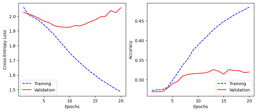
epochs = 20 #1min with 20epochs 128batch
history_MLP = MLP_model.fit(X_train, y_train, validation_data=(X_valid, y_valid),
                            batch_size=128, epochs=epochs)

MLP_model.save_weights("./checkpoints/MLP_10/MLP_10_TheOffice10") # Save the network's weights
#MLP_model.save("./checkpoints/MLP_10_model") #for saving the whole model object

loss_MLP, accuracy_MLP = MLP_model.evaluate(X_valid, y_valid)

print("Loss: ", loss_MLP)
print("Accuracy: ", accuracy_MLP)
Epoch 1/20
247/247 [==============================] - 3s 10ms/step - loss: 2.0617 - accuracy: 0.2724 - val_loss: 2.0262 - val_accuracy: 0.2693
Epoch 2/20
247/247 [==============================] - 2s 10ms/step - loss: 2.0083 - accuracy: 0.2742 - val_loss: 2.0154 - val_accuracy: 0.2693
Epoch 3/20
247/247 [==============================] - 2s 9ms/step - loss: 1.9923 - accuracy: 0.2746 - val_loss: 2.0024 - val_accuracy: 0.2694
Epoch 4/20
247/247 [==============================] - 2s 9ms/step - loss: 1.9709 - accuracy: 0.2801 - val_loss: 1.9850 - val_accuracy: 0.2780
Epoch 5/20
247/247 [==============================] - 2s 9ms/step - loss: 1.9414 - accuracy: 0.2980 - val_loss: 1.9673 - val_accuracy: 0.2894
Epoch 6/20
247/247 [==============================] - 2s 9ms/step - loss: 1.9078 - accuracy: 0.3169 - val_loss: 1.9563 - val_accuracy: 0.2955
Epoch 7/20
247/247 [==============================] - 2s 9ms/step - loss: 1.8723 - accuracy: 0.3369 - val_loss: 1.9357 - val_accuracy: 0.3094
Epoch 8/20
247/247 [==============================] - 2s 9ms/step - loss: 1.8324 - accuracy: 0.3526 - val_loss: 1.9282 - val_accuracy: 0.3132
Epoch 9/20
247/247 [==============================] - 2s 10ms/step - loss: 1.7921 - accuracy: 0.3749 - val_loss: 1.9253 - val_accuracy: 0.3152
Epoch 10/20
247/247 [==============================] - 2s 9ms/step - loss: 1.7518 - accuracy: 0.3884 - val_loss: 1.9251 - val_accuracy: 0.3161
Epoch 11/20
247/247 [==============================] - 2s 9ms/step - loss: 1.7167 - accuracy: 0.4016 - val_loss: 1.9360 - val_accuracy: 0.3167
Epoch 12/20
247/247 [==============================] - 2s 9ms/step - loss: 1.6846 - accuracy: 0.4140 - val_loss: 1.9344 - val_accuracy: 0.3194
Epoch 13/20
247/247 [==============================] - 2s 9ms/step - loss: 1.6530 - accuracy: 0.4276 - val_loss: 1.9460 - val_accuracy: 0.3257
Epoch 14/20
247/247 [==============================] - 2s 9ms/step - loss: 1.6236 - accuracy: 0.4386 - val_loss: 1.9630 - val_accuracy: 0.3217
Epoch 15/20
247/247 [==============================] - 2s 10ms/step - loss: 1.5973 - accuracy: 0.4487 - val_loss: 1.9750 - val_accuracy: 0.3141
Epoch 16/20
247/247 [==============================] - 2s 10ms/step - loss: 1.5708 - accuracy: 0.4562 - val_loss: 1.9956 - val_accuracy: 0.3258
Epoch 17/20
247/247 [==============================] - 2s 10ms/step - loss: 1.5492 - accuracy: 0.4646 - val_loss: 1.9995 - val_accuracy: 0.3234
Epoch 18/20
247/247 [==============================] - 2s 9ms/step - loss: 1.5270 - accuracy: 0.4719 - val_loss: 2.0382 - val_accuracy: 0.3231
Epoch 19/20
247/247 [==============================] - 2s 9ms/step - loss: 1.5051 - accuracy: 0.4785 - val_loss: 2.0247 - val_accuracy: 0.3181
Epoch 20/20
247/247 [==============================] - 2s 9ms/step - loss: 1.4870 - accuracy: 0.4852 - val_loss: 2.0573 - val_accuracy: 0.3195
247/247 [==============================] - 1s 2ms/step - loss: 2.0573 - accuracy: 0.3195
Loss:  2.0573484897613525
Accuracy:  0.3195078670978546
history_MLP_dict = history_MLP.history
history_MLP_dict.keys()

plot_training(history_MLP_dict)
char = 'Dwight' # ['Michael', 'Dwight', 'Jim', 'Pam', 'Andy', 'Kevin', 'Angela', 'Erin', 'Oscar', 'Ryan']
examples = list(TheOffice[TheOffice['speaker'] == char]['line'][1:20])

MLP_model.predict(examples)
print(predict_class(MLP_model, examples, main_characters))
nb_correct_pred = sum(predict_class(MLP_model, examples, main_characters) == char)/len(predict_class(BLSTM_model, examples, main_characters)
)
perc_correct_pred = np.array(nb_correct_pred).round(2)
perc_correct_pred
1/1 [==============================] - 0s 34ms/step
1/1 [==============================] - 0s 29ms/step

['Michael' 'Michael' 'Michael' 'Jim' 'Dwight' 'Michael' 'Dwight' 'Dwight'
 'Dwight' 'Dwight' 'Dwight' 'Michael' 'Michael' 'Dwight' 'Dwight' 'Dwight'
 'Dwight' 'Dwight' 'Dwight']

1/1 [==============================] - 0s 23ms/step
1/1 [==============================] - 0s 46ms/step

0.63
BiDirectionnal Long-Short Term Memory (BLSTM)
max_vocab = 10000
vectorize_layer = layers.TextVectorization(max_tokens=max_vocab, standardize='lower_and_strip_punctuation',
                                           output_mode='int', output_sequence_length=None)
vectorize_layer.adapt(X_train)
embedding_dim=50

# Using masking with 'mask_zero=True' to handle the variable sequence lengths in subsequent layers.

LSTM_model = tf.keras.Sequential([
    vectorize_layer,
    layers.Embedding(input_dim=len(vectorize_layer.get_vocabulary()), output_dim=embedding_dim,
                     embeddings_initializer='uniform', mask_zero=True),
    layers.LSTM(64),
    layers.Dense(64, activation='relu'),
    layers.Dense(n_classes, activation='softmax')
], name="LSTM_model")

BLSTM_model = tf.keras.Sequential([
    vectorize_layer,
    layers.Embedding(input_dim=len(vectorize_layer.get_vocabulary()), output_dim=embedding_dim,
                     embeddings_initializer='uniform', mask_zero=True),
    layers.Bidirectional(layers.LSTM(64), merge_mode='concat'),
    layers.Dense(n_classes, activation='softmax')
], name="BLSTM_model")

BLSTM2_model = tf.keras.Sequential([
    vectorize_layer,
    layers.Embedding(input_dim=len(vectorize_layer.get_vocabulary()), output_dim=embedding_dim,
                     embeddings_initializer='uniform', mask_zero=True),
    layers.Bidirectional(layers.LSTM(64,  return_sequences=True), merge_mode='concat'),
    layers.Bidirectional(layers.LSTM(32,  return_sequences=False), merge_mode='concat'),
    layers.Dense(64, activation='relu'),
    layers.Dropout(0.5),
    layers.Dense(n_classes, activation='softmax')
], name="BLSTM2_model")

BLSTM_model.compile(optimizer=optimizers.Adam(learning_rate=1e-4),
                    loss=losses.SparseCategoricalCrossentropy(from_logits=False),
                    metrics=['accuracy'])
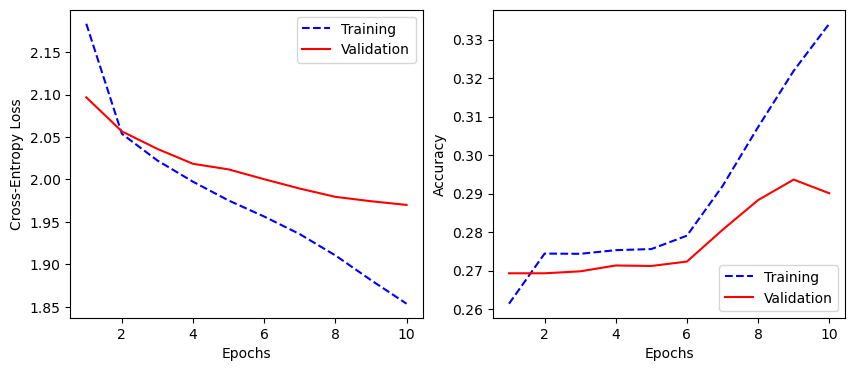
epochs = 10 #100
history_lstm = BLSTM_model.fit(X_train, y_train, validation_data=(X_valid, y_valid),
                               batch_size=128, epochs=epochs)

BLSTM_model.save_weights("./checkpoints/BLSTM_10/BLSTM_10")
#BLSTM_model.save("./checkpoints/BLSTM_10_model")
#BLSTM_model.load_weights("./checkpoints/BLSTM_10/BLSTM_10")
Epoch 1/10
247/247 [==============================] - 43s 150ms/step - loss: 2.1834 - accuracy: 0.2614 - val_loss: 2.0967 - val_accuracy: 0.2693
Epoch 2/10
247/247 [==============================] - 46s 186ms/step - loss: 2.0538 - accuracy: 0.2744 - val_loss: 2.0567 - val_accuracy: 0.2693
Epoch 3/10
247/247 [==============================] - 47s 192ms/step - loss: 2.0223 - accuracy: 0.2743 - val_loss: 2.0360 - val_accuracy: 0.2698
Epoch 4/10
247/247 [==============================] - 48s 196ms/step - loss: 1.9973 - accuracy: 0.2753 - val_loss: 2.0184 - val_accuracy: 0.2713
Epoch 5/10
247/247 [==============================] - 50s 202ms/step - loss: 1.9753 - accuracy: 0.2756 - val_loss: 2.0119 - val_accuracy: 0.2712
Epoch 6/10
247/247 [==============================] - 49s 199ms/step - loss: 1.9563 - accuracy: 0.2791 - val_loss: 2.0003 - val_accuracy: 0.2723
Epoch 7/10
247/247 [==============================] - 49s 198ms/step - loss: 1.9356 - accuracy: 0.2919 - val_loss: 1.9893 - val_accuracy: 0.2806
Epoch 8/10
247/247 [==============================] - 50s 204ms/step - loss: 1.9106 - accuracy: 0.3073 - val_loss: 1.9796 - val_accuracy: 0.2883
Epoch 9/10
247/247 [==============================] - 52s 211ms/step - loss: 1.8815 - accuracy: 0.3219 - val_loss: 1.9744 - val_accuracy: 0.2936
Epoch 10/10
247/247 [==============================] - 50s 203ms/step - loss: 1.8537 - accuracy: 0.3341 - val_loss: 1.9700 - val_accuracy: 0.2901
history_lstm_dict = history_lstm.history

test_loss_BLSTM, test_acc_BLSTM = BLSTM_model.evaluate(X_valid, y_valid)

print('Test Loss:', test_loss_BLSTM)
print('Test Accuracy:', test_acc_BLSTM)

plot_training(history_lstm_dict)
247/247 [==============================] - 3s 11ms/step - loss: 1.9700 - accuracy: 0.2901
Test Loss: 1.97004234790802
Test Accuracy: 0.2900811731815338
char = 'Dwight'
examples = list(TheOffice[TheOffice['speaker'] == char]['line'][1:20]) # ['Michael', 'Dwight', 'Jim', 'Pam', 'Andy', 'Kevin', 'Angela', 'Erin', 'Oscar', 'Ryan']

BLSTM_model.predict(examples)
print(predict_class(BLSTM_model, examples, main_characters))
nb_correct_pred = sum(predict_class(BLSTM_model, examples, main_characters) == char)/len(predict_class(BLSTM_model, examples, main_characters)
)
perc_correct_pred = np.array(nb_correct_pred).round(2)
perc_correct_pred
1/1 [==============================] - 0s 46ms/step
1/1 [==============================] - 0s 29ms/step

['Michael' 'Michael' 'Michael' 'Dwight' 'Dwight' 'Michael' 'Dwight'
 'Michael' 'Michael' 'Michael' 'Michael' 'Michael' 'Michael' 'Michael'
 'Dwight' 'Michael' 'Michael' 'Dwight' 'Dwight']

1/1 [==============================] - 0s 51ms/step
1/1 [==============================] - 0s 26ms/step

0.32
Conclusion
In this post, I have applied various ML and DL techniques to obtain some initial results on this quote classification task. The overall accuracy of each models fall in the [0.27-0.33] range. On one side, these look like bad results as the accuracy is fairly low. But on the other side, these results showcase a better guess than going purely random on 20 classes, or applying all the classes to the most common speaker (Michael). These results also represent just a first step in classifying the quotes. Indeed, much hyperparameter tuning and text preprocessing optimization can be done. The overall classifying accuracy should be able to increase.
The next paths I will investigate are among the following ones:
- Finetune the best models
- Add scene context
- Reduce the size of the set of main characters
- check other embeddings
- look for other DL methods more suited for such tasks
Work In Progress
Next Steps
Transfer Learning with keras
from transformers import AutoTokenizer, TFAutoModelForSequenceClassification

pretrained_name2 = "bert-base-cased" # e.g. "bert-base-cased" or "distilbert-base-uncased"

tokenizer = AutoTokenizer.from_pretrained(pretrained_name2)
model = TFAutoModelForSequenceClassification.from_pretrained(pretrained_name2, num_labels=n_classes)
model.summary()
model.layers[0].trainable = False
model.summary()
X_train_tok = dict(tokenizer(X_train.tolist(), padding=True, truncation=True, return_tensors="tf"))
X_valid_tok = dict(tokenizer(X_valid.tolist(), padding=True, truncation=True, return_tensors="tf"))
model.compile(optimizer=optimizers.Adam(learning_rate=3e-5),
              loss=losses.SparseCategoricalCrossentropy(from_logits=True),
              metrics=['accuracy'])
# The fit is very long without a GPU or a cloud service
epochs = 5
history_ft = model.fit(X_train_tok, y_train, validation_data=(X_valid_tok, y_valid),
                       batch_size=16, epochs=epochs)