Abstract
In this mini-project, we observe how different deep learning techniques affect a given model’s performance. In this context, we investigate the use of batch normalization, weight sharing and auxiliary losses to reduce computing time and model complexity, while achieving high performance.
Introduction
The increase in computational power has led to the development of deep neural networks, which have given way to unforeseen performances and increased scientific interest. However, training these networks is not an easy task. Problems related to overfitting, gradient vanishing or exploding and computational time has led researchers to focus on methods that could mitigate those problems. One of them is to use auxiliary losses to help back-propagating the gradient signal by adding small classifiers to early stage modules of a deep network. Their weighted losses is then summed to the loss of the main model. This was introduced by Google LeNet’s paper. On the other hand, weight sharing is a powerful tool that was introduced for the first time by scientists in 1985 that lets you reduce the number of free parameters in your model by making several connections that are controlled by the same parameter. This decreases the degree of freedom of a given model. Finally, we also make extensive use of batch normalization to stabilize the gradient during training. Without it, our models have shown to be unstable. The task at hand was to classify a pair of two handwritten digits from the MNIST dataset. Instead of the original images, we work with a pair of 14x14 grayscale images generated from the original dataset. With \(x_{j1}\) and \(x_{j2}\) the two digits of the pair \(x_j\), the class \(c\) is $$c_j = \unicode{x1D7D9}(x_1 ≤ x_2),$$ where \(\unicode{x1D7D9}\) is the indicator function. In other words, we classify the pair \(x_j\) as being 1 if the first digit is smaller or equal than the second digit, and 0 otherwise. To achieve that, we first focus on a basic ConvNet architecture with batch normalization (Baseline). Then, we propose another architecture, where the pair is passed hrough a siamese network in which each digit is trained with the same weights. For the siamese network, we evaluate the performance twice, once by optimizing the network with a linear combination of the weighted losses (Siamese2) and once using each branch of the siamese network to classify the digits separately (Siamese10).
Models
Baseline
The Baseline model consists of a convolutional layer with 2 channels as input and kernel size 4, a maximum pooling layer of kernel size 4, the ReLU activation function and a batch normalization layer; another convolutional layer with kernel size 4, ReLU and batch normalization. After the convolutional blocks, we added two fully connected layers with ReLU non-linearities and lastly a dense layer with two output units. This model was optimized using stochastic gradient descent (SGD) and the loss was computed using cross-entropy.
Siamese
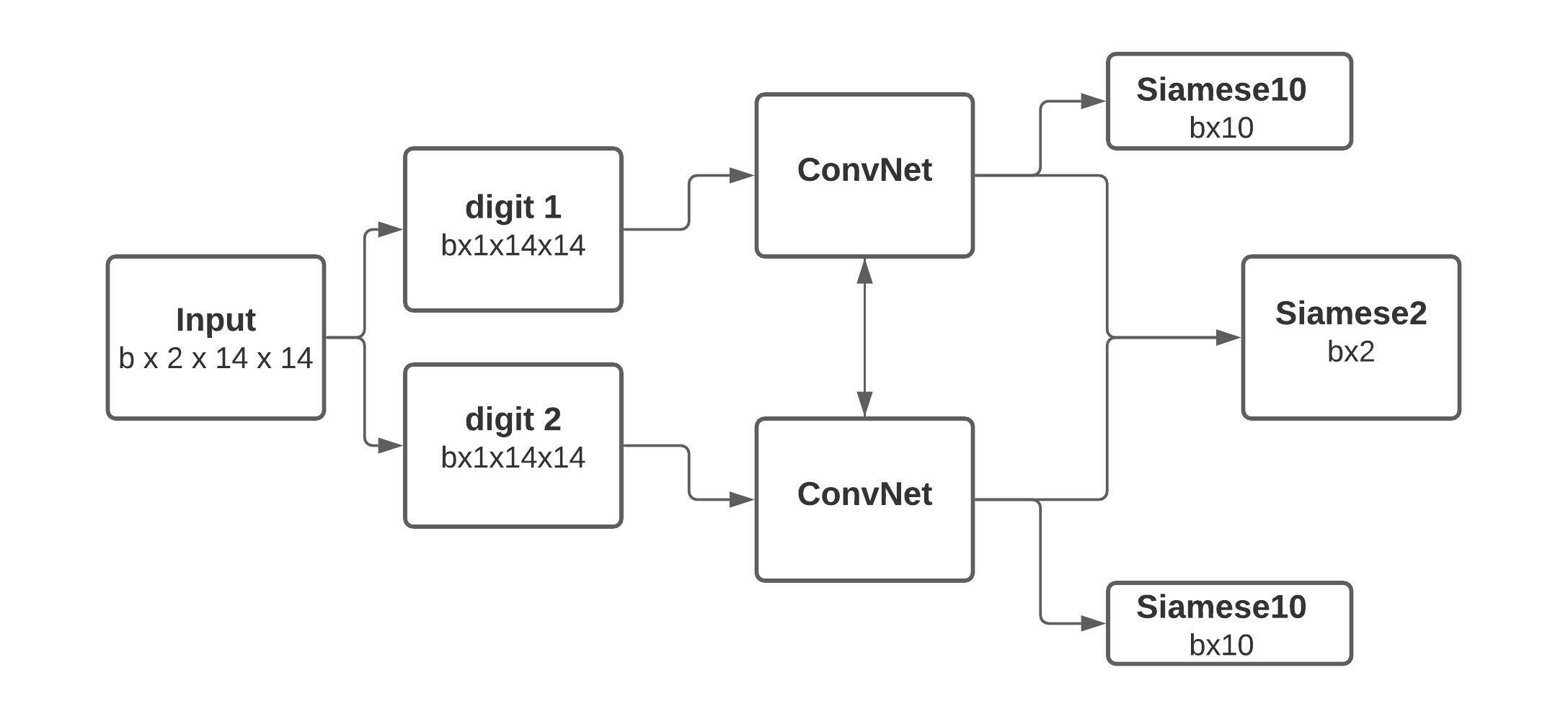
The Siamese network has a similar base as the baseline model. However, we now split the pair into two separate 1-channel images that will serve as the input of a ConvNet with shared weights. Each ConvNet has a convolutional layer with 1 channel as input, a maximum pooling layer, of kernel size 2, ReLU, batch normalization. The convolutional block is then repeated, but without the maximum pooling. Afterward, the output is passed on to a fully connected layer, the ReLU activation function, a batch normalization layer, a last dense linear layer with 10 outputs for the 10 different possible classes and the ReLU non-linearity. Finally, both branches are concatenated and passed on to a dense layer with two outputs and a ReLU activation function to get the final classification. Figure 1 illustrates the siamese architecture.
Results
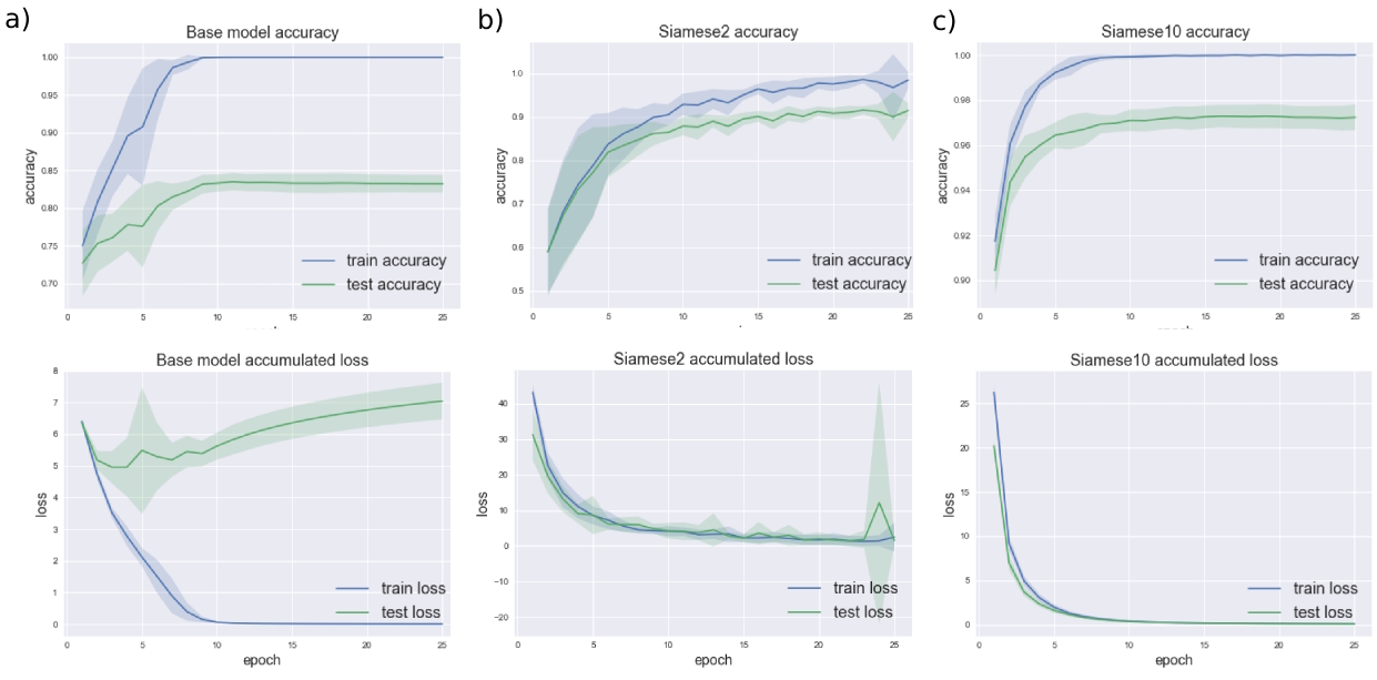
The two networks were tested with different architectures. Once the above-described architectures were retained, we performed a gridsearch and a 10-folds cross validation to find the optimal number of channels, units in the fully connected layers and the learning rate. The detailed implementation can be found in the gridsearch.py file. For Baseline, we found the optimal number of channels for the two convolutional layers to be 64 and the two fully connected linear layers have each 128 units. The optimal learning rate is η = 0.1. For Siamese2, when using the auxiliary losses to make a final prediction, we found that the optimal number of output channels for the first convolutional layer was 64 and 8 for the second. The fully connected layer has 64 units and uses the 10-classes and 2-classes losses equally. The optimal learning rate was found to be η = 1, which seems surprisingly high. At last, for Siamese10, where we only trained the network using the 10-classes losses, the optimal parameters where found to be 64 output channels for the first convolutional layer, 16 for the second, 64 units for the linear layer and a learning rate of η = 0.1. The accuracy and the accumulated loss are illustrated for the three models in Figure 2. The test accuracies computed on 10 independent datasets are presented in Table 1.
| Accuracy (%) | Std | |
|---|---|---|
| Baseline | 83.23 | 1.17 |
| Siamese2 | 91.50 | 1.65 |
| Siamese10 | 97.23 | 0.57 |
Discussion
We were surprised to see that the naive Baseline model performed relatively well when choosing optimal parameters. The Siamese2 model achieved a satisfying accuracy. However, we must observe that it is more unstable than the other models. Further work could focus on the apparent instability at epoch 24 which is driven by only 2 out of the 10 runs. One interesting thing to see is that the gradient was immediately recovered at the last epoch. More tests should be conducted to try to understand the cause of it. On the other hand, the Siamese10 model achieved the highest accuracy with the greatest stability. Basically, this model is trained to correctly recognize the correct class of each separate digit. We hypothesized, though, that Siamese2 would be able to, at least, match the 10-classes accuracy, but that is clearly not the case.
by René de CHAMPS, Olivier GROGNUZ & Thiago BORBA