Introduction
The task of this second project was to implement a mini deep-learning framework from scratch. The aim was to predict the class of a point depending on its position on a grid, the target being a circle in a square. The framework consists of a model which contains several Fully Connected Layers and activation functions that, with the help of a loss function and an optimizer, help us predict the class of each point in a set.
Framework
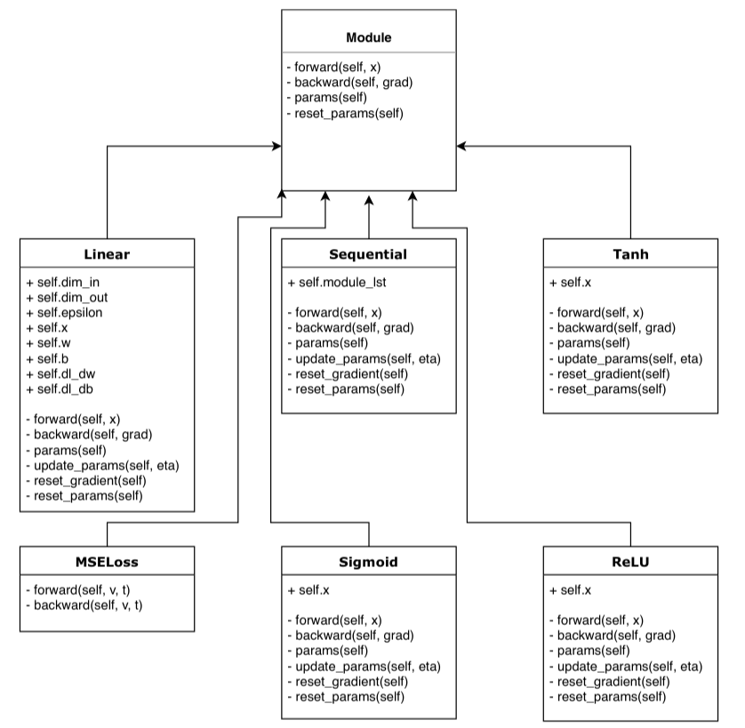
Our deep-learning framework consists of diverse classes spread across several files. We’ll briefly go through each of them to explain their content and use. Figure 1 depicts graphically our setup with all involved classes and their respective attributes.
model.py
This first python file contains the 2 general classes : Module and Sequential. The Module class is the overall unit from which further classes will inherit. It contains the 3 main methods: forward, backward and parameters. The sequential class is the model architecture. It gets hold of all layers and activation function we’ll further use and assesses the directives to take. It is the intermediary between the model and its components. Each methods in this class calls for the respective one in the subsequent layer or function.
linear.py
This file contains our standard fully connected layer class. This class starts off initializing the weights and biases matrices with their respective gradient. The forward method keeps a copy of the input then transforms it, at first, with the previously defined parameters. The backward method makes the necessary computations to obtain the partial derivative of the loss with respect to the parameters and the input. The SGD method updates, and so optimizes, the parameters using the previously computed partial derivatives. We also introduce a momentum term in the computation to help accelerate gradient towards the optimum point. Several methods were tried for the initialization of the first forward pass. When the parameters were initialized with a value sampled from a standard normal, our model was not able to converge and the gradients got stuck. For this reason, we switched to the Xavier initialization from PyTorch which allowed our network to train and seems to stabilize the gradients. Finally 2 methods are implemented to reset both the parameters if needed and the gradients matrices at every batch.
activation.py
We can find the 2 activation functions in this file. They both have a forward method transforming the inputs through their respective computations and the backward computing the derivative of the latter. The same goes for the Mean squared Error loss function with its forward and backward passes.
disk-generator.py
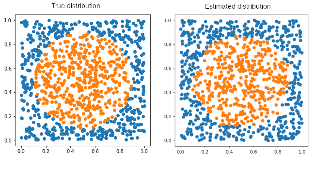
This disk generator function takes as input the desired number of points needed and provides 2 sets of input and target for the following exercise and delivers a set of points, assigning them to one of two classes, if the point is in the circle of a given diameter. Figure 1 illustrates the generated points.
Application
The final file test.py contains the executable to implement our mini-framework. We’ve automated the creation of the dataset and the implementation of a model containing 3 fully connected layers of size 25 with 2 ReLU activations and 2 Tanh activations. The model trains on a dataset of 1000 points and tests the prediction on a set of equal size. The optimization is done through a Stochastic Gradient Descent with momentum 0.9, and the help of a Mean squared Error function. Working through the data 100 times with batches of size 100, we get in average test errors ranging from 2% to 5%. Figure 2 clearly shows that our model performs well for this type of data. The decision boundary is able to capture the true distribution well.
by René de CHAMPS, Olivier GROGNUZ & Thiago BORBA