I. Introduction: Description of the data set, imports, notebook structure
Description of the dataset
In this analysis, we’re looking at a dataset containing tweets : short messages posted by users on www.twitter.com. We’re aiming at modelling and predicting the sentiment, whether positive or negative, of each tweet. The sentiment of the tweet was based on whether each tweet contained a happy “:)” or sad “:(“ smiley. These smileys have been removed from the tweets beforehand.
Notebook structure
We’ll proceed in this analysis by making a first exploratory data analysis in which we’ll take an overall look at our data to get a first intuition on how to approach the modelling. Then, we’ll apply different modelling approach and try to compare them using predictive scoring. Finally, after tuning up our best model to get the best possible training fit, we’ll apply our model on the test dataset which will serve as our final prediction result. Furthermore, we added an appendix at the end containing a long and perilous attempt on using BERT model.
Libraries
Let’s first load the various libraries needed for this analysis.
import matplotlib.pyplot as plt
%matplotlib inline
import numpy as np
import pandas as pd
import keras.backend as K

from numpy import array, asarray, zeros
from sklearn.model_selection import KFold, train_test_split, GridSearchCV
from sklearn.pipeline import Pipeline
from sklearn.linear_model import SGDClassifier, LogisticRegression
from sklearn.preprocessing import StandardScaler
from sklearn.svm import LinearSVC
from sklearn.naive_bayes import MultinomialNB
from sklearn.feature_extraction.text import CountVectorizer, TfidfTransformer, TfidfVectorizer
from sklearn.metrics import accuracy_score, confusion_matrix, classification_report

from keras.preprocessing import sequence
from keras.preprocessing.text import one_hot, Tokenizer
from keras.preprocessing.sequence import pad_sequences
from keras.layers import GlobalMaxPooling1D, Conv1D, LSTM, Flatten, Dense, Embedding, MaxPooling1D
from keras.layers.core import Activation, Dropout, Dense
from keras.layers.embeddings import Embedding
from keras.layers.convolutional import MaxPooling1D
from keras.models import Sequential
from keras.utils import np_utils

import nltk
from nltk.corpus import stopwords
from nltk.tokenize import word_tokenize
import re, string

import seaborn as sns
sns.set(style="darkgrid")
sns.set(font_scale=1.3)

from pprint import pprint
from time import time
import logging
Import
We then import the training dataset under the name “emote”.
emote = pd.read_csv("MLUnige2021_train.csv",index_col=0)
print("Dataset shape:", emote.shape)
Dataset shape: (1280000, 6)
II. Exploratory Data Analysis & Feature Engineering
First look at the data
Now that we’ve imported our training dataset, let’s take a first look into it.
emote.head()
| Id | emotion | tweet_id | date | lyx_query | user | text |
|---|---|---|---|---|---|---|
| 0 | 1 | 2063391019 | Sun Jun 07 02:28:13 PDT 2009 | NO_QUERY | BerryGurus | @BreeMe more time to play with you BlackBerry ... |
| 1 | 0 | 2000525676 | Mon Jun 01 22:18:53 PDT 2009 | NO_QUERY | peterlanoie | Failed attempt at booting to a flash drive. Th... |
| 2 | 0 | 2218180611 | Wed Jun 17 22:01:38 PDT 2009 | NO_QUERY | will_tooker | @msproductions Well ain't that the truth. Wher... |
| 3 | 1 | 2190269101 | Tue Jun 16 02:14:47 PDT 2009 | NO_QUERY | sammutimer | @Meaghery cheers Craig - that was really sweet... |
| 4 | 0 | 2069249490 | Sun Jun 07 15:31:58 PDT 2009 | NO_QUERY | ohaijustin | I was reading the tweets that got send to me w... |
This dataset contains not only the tweets and its corresponding emotions, but also the username of the sender, the date at which it was sent and a last column which indicates if a specific query was used in processing the data.
print("Missing values in our data :", emote.isna().sum().sum())
# No missing values

found = emote['lyx_query'].str.contains('NO_QUERY')
print("Instances of NO_QUERY in column 'lyx_query':", found.count())
# Full of "NO_QUERY"
Missing values in our data : 0
Instances of NO_QUERY in column 'lyx_query': 1280000
Our dataset doesn’t contain any missing values. Moreover, we observe that the column ‘lyx_query’ is full of the same statement ‘NO_QUERY’. Thus, this variable is of no use in the predictive aim of our model since it doesn’t make any discrimination between any tweet.
sns.catplot(x="emotion", data=emote, kind="count", height=6, aspect=1.5, palette="PuBuGn_d")
plt.show();
print("Number of positive tweets :", sum(emote["emotion"] == 1))
print("Number of negative tweets :", sum(emote["emotion"] == 0))
# About 50/50 positive and negative tweets
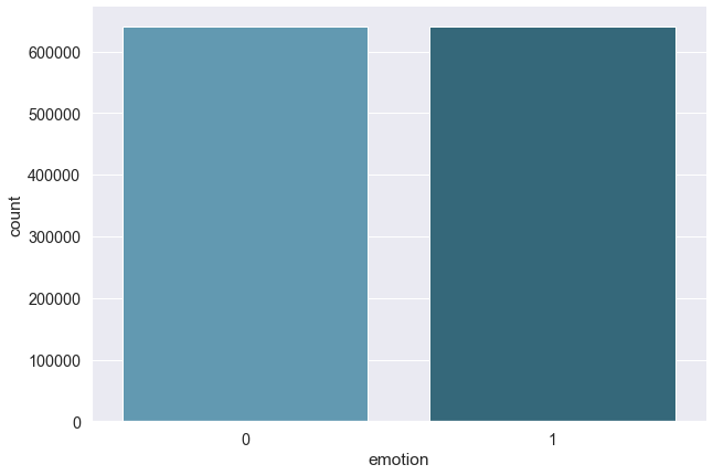
Number of positive tweets : 640118
Number of negative tweets : 639882
We are training on a pretty balanced dataset with as much positive and negative tweets. This will let us perform train/test split without the need of stratifying.
print("Number of different tweet id :", emote["tweet_id"].nunique()) # 1069 tweets have had same id ??
print("Number of different users :", emote["user"].nunique()) # 574.114 different users
print("Number of users that tweeted only once :", sum(emote["user"].value_counts() == 1)) # 365.446 users tweeted once
print("Various users and their number of posted tweets :")
print(emote["user"].value_counts()) # some of them commented a lot
Number of different tweet id : 1278931
Number of different users : 574114
Number of users that tweeted only once : 365446
Various users and their number of posted tweets :
lost_dog          446
webwoke           292
tweetpet          239
VioletsCRUK       234
mcraddictal       226
                 ...
anne_ccj            1
JocelynG42          1
wkdpstr             1
Strawberry_Sal      1
MichalMM            1
Name: user, Length: 574114, dtype: int64
About a quarter of the twitter users in our training dataset only tweeted once during that period, while some of them went as far as tweeting several hundred times.
5 Most talkative users data
emote[emote["user"] == "lost_dog"].head() # SPAM : all the 446 same message "@random_user I am lost. Please help me find a good home."
| Id | emotion | tweet_id | date | lyx_query | user | text |
|---|---|---|---|---|---|---|
| 8229 | 0 | 2209419659 | Wed Jun 17 10:22:06 PDT 2009 | NO_QUERY | lost_dog | @JamieDrokan I am lost. Please help me find a ... |
| 9527 | 0 | 2328965183 | Thu Jun 25 10:11:34 PDT 2009 | NO_QUERY | lost_dog | @W_Hancock I am lost. Please help me find a go... |
| 10645 | 0 | 2072079020 | Sun Jun 07 20:21:54 PDT 2009 | NO_QUERY | lost_dog | @miznatch I am lost. Please help me find a goo... |
| 14863 | 0 | 2214285766 | Wed Jun 17 16:31:38 PDT 2009 | NO_QUERY | lost_dog | @kgustafson I am lost. Please help me find a g... |
| 16723 | 0 | 1696136174 | Mon May 04 07:41:03 PDT 2009 | NO_QUERY | lost_dog | @kneeon I am lost. Please help me find a good ... |
emote[emote["user"] == "webwoke"].head() # SPAM : making request to visit some random website (commercial bot ?)
#emote[emote["user"] == "webwoke"].sum() # 68/292 positive messages
| Id | emotion | tweet_id | date | lyx_query | user | text |
|---|---|---|---|---|---|---|
| 19553 | 0 | 2067697514 | Sun Jun 07 12:48:05 PDT 2009 | NO_QUERY | webwoke | come on... drop by 1 44. blogtoplist.com |
| 24144 | 0 | 2072285184 | Sun Jun 07 20:44:08 PDT 2009 | NO_QUERY | webwoke | owww god, drop by 18 57. blogspot.com |
| 25988 | 0 | 2055206809 | Sat Jun 06 08:54:04 PDT 2009 | NO_QUERY | webwoke | F**K! drop by 1 97. zimbio.com |
| 28219 | 1 | 2053451192 | Sat Jun 06 04:36:04 PDT 2009 | NO_QUERY | webwoke | uhuiii... move up by 1 69. hubpages.com |
| 28597 | 1 | 2066463084 | Sun Jun 07 10:34:05 PDT 2009 | NO_QUERY | webwoke | GoGoGo... move up by 1 13. slideshare.net |
emote[emote["user"] == "tweetpet"].head() # SPAM : 239 messages asking to "@someone_else Clean me"
| Id | emotion | tweet_id | date | lyx_query | user | text |
|---|---|---|---|---|---|---|
| 11130 | 0 | 1676425868 | Fri May 01 22:00:38 PDT 2009 | NO_QUERY | tweetpet | @CeladonNewTown Clean Me! |
| 13494 | 0 | 1573611322 | Tue Apr 21 02:00:03 PDT 2009 | NO_QUERY | tweetpet | @chromachris Clean Me! |
| 17443 | 0 | 1676426980 | Fri May 01 22:00:49 PDT 2009 | NO_QUERY | tweetpet | @Kamryn6179 Clean Me! |
| 23973 | 0 | 1677423044 | Sat May 02 02:00:12 PDT 2009 | NO_QUERY | tweetpet | @greenbizdaily Clean Me! |
| 33463 | 0 | 1676426375 | Fri May 01 22:00:43 PDT 2009 | NO_QUERY | tweetpet | @ANALOVESTITO Clean Me! |
emote[emote["user"] == "VioletsCRUK"].sum() # 180/234 positive messages
emote[emote["user"] == "VioletsCRUK"].head()
| Id | emotion | tweet_id | date | lyx_query | user | text |
|---|---|---|---|---|---|---|
| 8319 | 0 | 2057611341 | Sat Jun 06 13:19:41 PDT 2009 | NO_QUERY | VioletsCRUK | @marginatasnaily lol i was chucked of 4 times ... |
| 9102 | 1 | 1573700635 | Tue Apr 21 02:26:06 PDT 2009 | NO_QUERY | VioletsCRUK | @highdigi Nothing worse! Rain has just started... |
| 16570 | 1 | 1980137710 | Sun May 31 05:49:01 PDT 2009 | NO_QUERY | VioletsCRUK | Will catch up with yas later..goin for a solid... |
| 37711 | 1 | 1881181047 | Fri May 22 03:52:11 PDT 2009 | NO_QUERY | VioletsCRUK | @Glasgowlassy lol oh that's a big buffet of ha... |
| 37909 | 0 | 2067636547 | Sun Jun 07 12:41:40 PDT 2009 | NO_QUERY | VioletsCRUK | @jimkerr09 That was a really lovely tribute to... |
emote[emote["user"] == "mcraddictal"].sum() # 54/226 positive messages
emote[emote["user"] == "mcraddictal"].head()
| Id | emotion | tweet_id | date | lyx_query | user | text |
|---|---|---|---|---|---|---|
| 2337 | 0 | 2059074446 | Sat Jun 06 16:11:42 PDT 2009 | NO_QUERY | mcraddictal | @MyCheMicALmuse pleaseeee tell me? -bites nail... |
| 2815 | 0 | 1968268387 | Fri May 29 21:05:43 PDT 2009 | NO_QUERY | mcraddictal | @MCRmuffin |
| 7448 | 0 | 2052420061 | Sat Jun 06 00:40:11 PDT 2009 | NO_QUERY | mcraddictal | @chemicalzombie dont make me say it you know. |
| 10092 | 0 | 2061250826 | Sat Jun 06 20:29:01 PDT 2009 | NO_QUERY | mcraddictal | @NoRaptors noooooo begging i hate that. I'm s... |
| 13533 | 0 | 1981070459 | Sun May 31 08:20:52 PDT 2009 | NO_QUERY | mcraddictal | @Boy_Kill_Boy so was haunting in ct. That mov... |
Out of the 5 users that tweeted the most, it seems like 3 of them are some kind of bot or spam bot. The 4th and 5th ones seem to be random users from which we got a lot tweets in the database. All these users show pattern in their sent tweets. Indeed, they tend to send messages that are not balanced towards their emotion. ‘Lost_dog’ and ‘tweetpet’ both sent only negative tweets out of hundreds of them. ‘webwoke’ and ‘mcraddictal’ also sent largely negative tweets while ‘VioletsCRUK’ sent mostly positive tweets. We’ll take this information into account when trying to classify further tweets.
emote = emote[['emotion', 'user', 'text']]
emote.head()
| Id | emotion | user | text |
|---|---|---|---|
| 0 | 1 | BerryGurus | @BreeMe more time to play with you BlackBerry ... |
| 1 | 0 | peterlanoie | Failed attempt at booting to a flash drive. Th... |
| 2 | 0 | will_tooker | @msproductions Well ain't that the truth. Wher... |
| 3 | 1 | sammutimer | @Meaghery cheers Craig - that was really sweet... |
| 4 | 0 | ohaijustin | I was reading the tweets that got send to me w... |
We add a column with the number of words per tweet:
emote['length'] = emote['text'].apply(lambda x: len(x.split(' ')))
emote.head()
max_tweet = max(emote["length"])
print('Largest tweet length:', max_tweet)
Largest tweet length: 110
Symbols
Make text lowercase, remove text in square brackets, remove links, remove punctuation, and remove words containing numbers:
def clean_text(text):
    text = str(text).lower()
    text = re.sub('\[.*?\]', '', text)
    text = re.sub('https?://\S+|www\.\S+', '', text)
    text = re.sub('<.*?>+', '', text)
    text = re.sub('[%s]' % re.escape(string.punctuation), '', text)
    text = re.sub('\n', '', text)
    text = re.sub('\w*\d\w*', '', text)

    return text
emote['text_clean'] = emote['text'].apply(clean_text) #maybe remove the name with the @
emote.head()
| Id | emotion | tweet_id | date | lyx_query | user | text | text_clean |
|---|---|---|---|---|---|---|---|
| 0 | 1 | 2063391019 | Sun Jun 07 02:28:13 PDT 2009 | NO_QUERY | BerryGurus | @BreeMe more time to play with you BlackBerry ... | breeme more time to play with you blackberry t... |
| 1 | 0 | 2000525676 | Mon Jun 01 22:18:53 PDT 2009 | NO_QUERY | peterlanoie | Failed attempt at booting to a flash drive. Th... | failed attempt at booting to a flash drive the... |
| 2 | 0 | 2218180611 | Wed Jun 17 22:01:38 PDT 2009 | NO_QUERY | will_tooker | @msproductions Well ain't that the truth. Wher... | msproductions well aint that the truth whered ... |
| 3 | 1 | 2190269101 | Tue Jun 16 02:14:47 PDT 2009 | NO_QUERY | sammutimer | @Meaghery cheers Craig - that was really sweet... | meaghery cheers craig that was really sweet o... |
| 4 | 0 | 2069249490 | Sun Jun 07 15:31:58 PDT 2009 | NO_QUERY | ohaijustin | I was reading the tweets that got send to me w... | i was reading the tweets that got send to me w... |
Stopwords
Remove stopwords (a list of not useful english words like ‘the’, ‘at’, etc.). It allows us to reduce dimension of the data when tokenizing.
stop_words = stopwords.words('english')
more_stopwords = ['u', 'im', 'c']
stop_words = stop_words + more_stopwords

def remove_stopwords(text):
    text = ' '.join(word for word in text.split(' ') if word not in stop_words)
    return text

emote['text_clean'] = emote['text_clean'].apply(remove_stopwords)
emote.head()
| Id | emotion | tweet_id | date | lyx_query | user | text | text_clean |
|---|---|---|---|---|---|---|---|
| 0 | 1 | 2063391019 | Sun Jun 07 02:28:13 PDT 2009 | NO_QUERY | BerryGurus | @BreeMe more time to play with you BlackBerry ... | breeme time play blackberry |
| 1 | 0 | 2000525676 | Mon Jun 01 22:18:53 PDT 2009 | NO_QUERY | peterlanoie | Failed attempt at booting to a flash drive. Th... | failed attempt booting flash drive failed atte... |
| 2 | 0 | 2218180611 | Wed Jun 17 22:01:38 PDT 2009 | NO_QUERY | will_tooker | @msproductions Well ain't that the truth. Wher... | msproductions well aint truth whered damn auto... |
| 3 | 1 | 2190269101 | Tue Jun 16 02:14:47 PDT 2009 | NO_QUERY | sammutimer | @Meaghery cheers Craig - that was really sweet... | meaghery cheers craig really sweet reply pumped |
| 4 | 0 | 2069249490 | Sun Jun 07 15:31:58 PDT 2009 | NO_QUERY | ohaijustin | I was reading the tweets that got send to me w... | reading tweets got send lying phone face dropp... |
Stemming/ Lematization
Stemming cuts off prefixes and suffixes (ex: laziness -> lazi). Lemma converts words (ex: writing, writes) into its radical (ex: write).
stemmer = nltk.SnowballStemmer("english")

def stemm_text(text):
    text = ' '.join(stemmer.stem(word) for word in text.split(' '))
    return text
emote['text_clean'] = emote['text_clean'].apply(stemm_text)
emote.head()
| Id | emotion | tweet_id | date | lyx_query | user | text | text_clean |
|---|---|---|---|---|---|---|---|
| 0 | 1 | 2063391019 | Sun Jun 07 02:28:13 PDT 2009 | NO_QUERY | BerryGurus | @BreeMe more time to play with you BlackBerry ... | breem time play blackberri |
| 1 | 0 | 2000525676 | Mon Jun 01 22:18:53 PDT 2009 | NO_QUERY | peterlanoie | Failed attempt at booting to a flash drive. Th... | fail attempt boot flash drive fail attempt swi... |
| 2 | 0 | 2218180611 | Wed Jun 17 22:01:38 PDT 2009 | NO_QUERY | will_tooker | @msproductions Well ain't that the truth. Wher... | msproduct well aint truth where damn autolock ... |
| 3 | 1 | 2190269101 | Tue Jun 16 02:14:47 PDT 2009 | NO_QUERY | sammutimer | @Meaghery cheers Craig - that was really sweet... | meagheri cheer craig realli sweet repli pump |
| 4 | 0 | 2069249490 | Sun Jun 07 15:31:58 PDT 2009 | NO_QUERY | ohaijustin | I was reading the tweets that got send to me w... | read tweet got send lie phone face drop ampit ... |
Wordclouds
#pip install wordcloud
from wordcloud import WordCloud
from PIL import Image
twitter_mask = np.array(Image.open('user.jpeg'))
wc = WordCloud(
background_color='white',
max_words=200,
mask=twitter_mask,
)
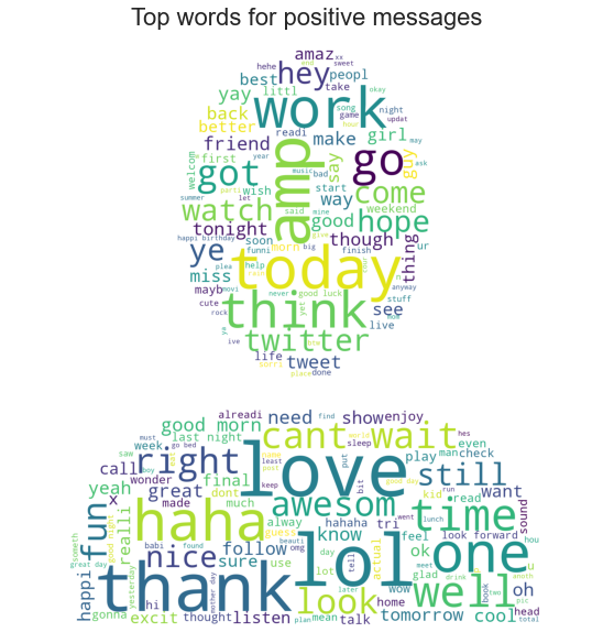
wc.generate(' '.join(text for text in emote.loc[emote['emotion'] == 1, 'text_clean']))
plt.figure(figsize=(18,10))
plt.title('Top words for positive messages',
fontdict={'size': 22, 'verticalalignment': 'bottom'})
plt.imshow(wc)
plt.axis("off")
plt.show()
twitter_mask = np.array(Image.open('user.jpeg'))

wc = WordCloud(
    background_color='white',
    max_words=200,
    mask=twitter_mask,
)
wc.generate(' '.join(text for text in emote.loc[emote['emotion'] == 0, 'text_clean']))
plt.figure(figsize=(18,10))
plt.title('Top words for negative messages',
          fontdict={'size': 22,  'verticalalignment': 'bottom'})
plt.imshow(wc)
plt.axis("off")
plt.show()
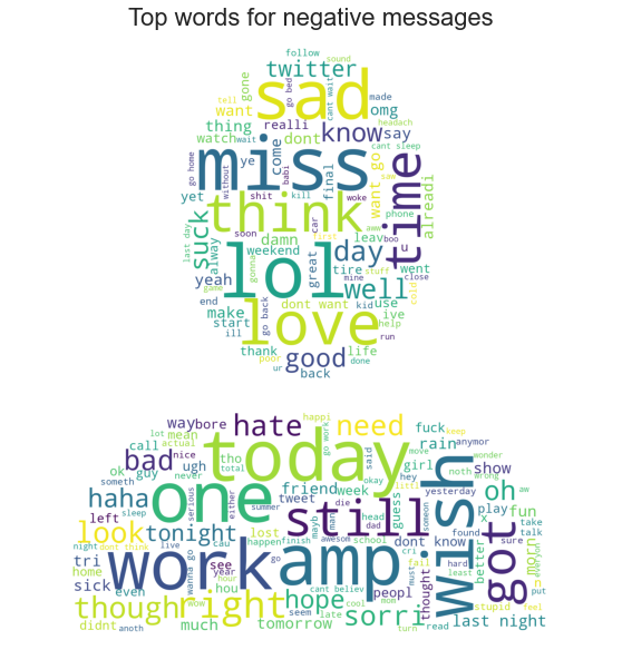
A nice representation of the most used words in each sentiment-type of messages
Now that we’ve taken a good first look at our data. We’ll try to compute some models. Since we’re trying to predict a binary outcome that is the sentiment of a given tweet, we’ll proceed with classification modelling. In order to do so, we first need to transform our text data into digits so that we can apply our models. We do so by using techniques that transform our data into numbers then work on the words frequency. As we were led to believe from the 5 most talkative (+ we compared models with and without) that usernames are good source of information towards predicting further sentiment (in this dataset), we combine the text and username as our predictors for further modelling.
emote_cut = emote.drop(emote.index[640000:1280000])
print("Cropped dataset shape:", emote_cut.shape)
X_train, X_test, y_train, y_test = train_test_split((emote.text + emote.user), emote.emotion, test_size=0.1, random_state=37)
print("First 5 entries of training dataset :", X_train.head())
Feature Engineering : Bag of words
The Vectorization and TF-IDF method
We will extract the numerical features of our text content using a first tool that will vectorize our corpus then a second one that will take into account the frequency of appearance of our words tokens.
First, we make use of CountVectorizer. This method tokenizes strings of words by transforming them into tokens (using white spaces as token separators)
Using CountVectorizer to tokenize and count the occurrences of words in our text dataset.
count_vect = CountVectorizer(ngram_range=(1, 3), token_pattern=r'\b\w+\b', min_df=1)
X_train_counts = count_vect.fit_transform(X_train)
X_train_counts.shape
Now we reweight the words counts through TF-IDF so that they can be used by classifier methods.
tfidftransformer = TfidfTransformer()
X_train_final = tfidftransformer.fit_transform(X_train_counts)
X_train_final.shape
III. Model Selection
The aim of this project is to learn from our tweet training dataset in order to being able to classify new tweets as being of positive or negative emotion. This is a classification task with binary outcome. There are several models that we’ve seen in class that can be of help here. We decided to present you our 3 best classification regression models. This is followed by attempts at building a Neural Network model that could predict better the tweet sentiment.
Preprocessing Effectiveness
We will compare the effectiveness of preprocessing the data in the aim of increasing our prediction accuracy by comparing 2 models respectively including pre-processed data and unprocessed data.
Here’s a first logistic model fit on 50 000 observations, with preprocessing :
pipeline_log = Pipeline([
    ('vect', CountVectorizer()),
    ('tfidf', TfidfTransformer()),
    ('log', LogisticRegression()),
])
emote_cut = emote.drop(emote.index[50000:1280000])
X_train, X_test, y_train, y_test = train_test_split((emote_cut.text + emote_cut.user), emote_cut.emotion, test_size=0.1, random_state=37)

grid_search_log = GridSearchCV(pipeline_log, parameters_log, n_jobs=-1, verbose=1)

print("Performing grid search...")
print("pipeline:", [name for name, _ in pipeline_log.steps])
print("parameters:")
pprint(parameters_log)
t0 = time()
grid_search_log.fit(emote_cut.text_clean, emote_cut.emotion)
print("done in %0.3fs" % (time() - t0))
print()

print("Best score: %0.3f" % grid_search_log.best_score_)
print("Best parameters set:")
best_parameters = grid_search_log.best_estimator_.get_params()
for param_name in sorted(parameters_log.keys()):
    print("\t%s: %r" % (param_name, best_parameters[param_name]))
Performing grid search...
pipeline: ['vect', 'tfidf', 'log']
parameters:
{'log__C': (0.5, 0.75, 1.0),
 'log__penalty': ('l2',),
 'vect__ngram_range': ((1, 2), (1, 3))}
Fitting 5 folds for each of 6 candidates, totaling 30 fits
done in 45.296s

Best score: 0.760
Best parameters set:
	log__C: 1.0
	log__penalty: 'l2'
	vect__ngram_range: (1, 2)
We achieved a prediction score of 76% using logistic regression on 50 000 observations. Let’s now compare this score with the one using the unprocessed data :
pipeline_log = Pipeline([
    ('vect', CountVectorizer()),
    ('tfidf', TfidfTransformer()),
    ('log', LogisticRegression()),
])
emote_cut = emote.drop(emote.index[50000:1280000])
X_train, X_test, y_train, y_test = train_test_split((emote_cut.text + emote_cut.user), emote_cut.emotion, test_size=0.1, random_state=37)

grid_search_log = GridSearchCV(pipeline_log, parameters_log, n_jobs=-1, verbose=1)

print("Performing grid search...")
print("pipeline:", [name for name, _ in pipeline_log.steps])
print("parameters:")
pprint(parameters_log)
t0 = time()
grid_search_log.fit(emote_cut.text, emote_cut.emotion)
print("done in %0.3fs" % (time() - t0))
print()

print("Best score: %0.3f" % grid_search_log.best_score_)
print("Best parameters set:")
best_parameters = grid_search_log.best_estimator_.get_params()
for param_name in sorted(parameters_log.keys()):
    print("\t%s: %r" % (param_name, best_parameters[param_name]))
Performing grid search...
pipeline: ['vect', 'tfidf', 'log']
parameters:
{'log__C': (0.5, 0.75, 1.0),
 'log__penalty': ('l2',),
 'vect__ngram_range': ((1, 2), (1, 3))}
Fitting 5 folds for each of 6 candidates, totaling 30 fits
done in 68.993s

Best score: 0.777
Best parameters set:
	log__C: 1.0
	log__penalty: 'l2'
	vect__ngram_range: (1, 2)
We achieved a prediction score of 77.7% with 50 000 observations using logistic regression on unprocessed data. We observe that the preprocess is actually hurting our prediction accuracy.
In this case, we fitted the same models once without any kind of preprocess and a second time using various preprocess methods. Selecting each of these methods separately (not shown here) guided us in the same direction. We found no preprocess techniques worth adding in the aim of better prediction accuracy for this dataset.
Support Vector Machine (SVM)
One of the most efficient prediction tool we saw in class was Support Vector Machine. Here we fit it trying different set of tuning parameters. First let’s define a pipeline which includes the tokenizer, the term weighting scheme and our SVM model.
pipeline_svm = Pipeline([
    ('vect', CountVectorizer()),
    ('tfidf', TfidfTransformer()),
    ('svm', LinearSVC()),
])
Then, we make a small dictionary containing all the parameters we want to test during our Cross-Validation. (We have already fitted dozens of models with even larger sets. In order not to make it run several hours, we’ve decided to crop this parameter set to its few main components).
parameters_svm = {
    # 'vect__max_df': (0.4, 0.5),
    # 'vect__max_features': (None, 50000, 200000, 400000),
    'vect__ngram_range': ((1, 2), (1, 3),),
    #'svm__penalty': ('l2', 'elasticnet'),
    # 'svm__loss': ('squared_hinge',),
    'svm__C': (0.6, 0.7, 0.8),
}
Then comes the Cross-Validation part. Here, all possible combination of parameters are tested on our training data in the aim of finding the parameter set that yields the best possible prediction score on various K-Folds. Here is the output for 320 000 observations :
'''emote_cut = emote.drop(emote.index[3200000:1280000])
X_train, X_test, y_train, y_test = train_test_split((emote_cut.text + emote_cut.user), emote_cut.emotion, test_size=0.1, random_state=37)'''

grid_search_svm = GridSearchCV(pipeline_svm, parameters_svm, verbose=1)

print("Performing grid search...")
print("pipeline:", [name for name, _ in pipeline_svm.steps])
print("parameters:")
pprint(parameters_svm)
t0 = time()
grid_search_svm.fit(X_train, y_train)
print("done in %0.3fs" % (time() - t0))
print()

print("Best score: %0.3f" % grid_search_svm.best_score_)
print("Best parameters set:")
best_parameters = grid_search_svm.best_estimator_.get_params()
for param_name in sorted(parameters_svm.keys()):
    print("\t%s: %r" % (param_name, best_parameters[param_name]))
Performing grid search...
pipeline: ['vect', 'tfidf', 'svm']
parameters:
{'svm__C': (0.7,),
 'svm__penalty': ('l2',),
 'vect__max_features': (None, 50000, 200000, 400000),
 'vect__ngram_range': ((1, 3),)}
Fitting 5 folds for each of 4 candidates, totaling 20 fits
done in 875.074s

Best score: 0.815
Best parameters set:
	svm__C: 0.7
	svm__penalty: 'l2'
	vect__max_features: None
	vect__ngram_range: (1, 3)
And here the one for computing on 640 000 observations
'''emote_cut = emote.drop(emote.index[6400000:1280000])
X_train, X_test, y_train, y_test = train_test_split((emote_cut.text + emote_cut.user), emote_cut.emotion, test_size=0.1, random_state=37)'''

grid_search_svm = GridSearchCV(pipeline_svm, parameters_svm, verbose=1)

print("Performing grid search...")
print("pipeline:", [name for name, _ in pipeline_svm.steps])
print("parameters:")
pprint(parameters_svm)
t0 = time()
grid_search_svm.fit(X_train, y_train)
print("done in %0.3fs" % (time() - t0))
print()

print("Best score: %0.3f" % grid_search_svm.best_score_)
print("Best parameters set:")
best_parameters = grid_search_svm.best_estimator_.get_params()
for param_name in sorted(parameters_svm.keys()):
    print("\t%s: %r" % (param_name, best_parameters[param_name]))
Performing grid search...
pipeline: ['vect', 'tfidf', 'svm']
parameters:
{'svm__C': (0.6, 0.7, 0.8), 'vect__ngram_range': ((1, 2), (1, 3))}
Fitting 5 folds for each of 6 candidates, totaling 30 fits
done in 3555.632s

Best score: 0.830
Best parameters set:
	svm__C: 0.8
	vect__ngram_range: (1, 3)
Using half of our training dataset to fit some Cross validation models, we obtain a score of 83% on this SVM model with the above parameters. This is one of the best predictions we were able to make.
In order to compare with the following methods, we fitted this additional SVM on 100 000 observations :
emote_cut = emote.drop(emote.index[100000:1280000])
X_train, X_test, y_train, y_test = train_test_split((emote_cut.text + emote_cut.user), emote_cut.emotion, test_size=0.1, random_state=37)

grid_search_svm = GridSearchCV(pipeline_svm, parameters_svm, verbose=1)

print("Performing grid search...")
print("pipeline:", [name for name, _ in pipeline_svm.steps])
print("parameters:")
pprint(parameters_svm)
t0 = time()
grid_search_svm.fit(X_train, y_train)
print("done in %0.3fs" % (time() - t0))
print()

print("Best score: %0.3f" % grid_search_svm.best_score_)
print("Best parameters set:")
best_parameters = grid_search_svm.best_estimator_.get_params()
for param_name in sorted(parameters_svm.keys()):
    print("\t%s: %r" % (param_name, best_parameters[param_name]))
Performing grid search...
pipeline: ['vect', 'tfidf', 'svm']
parameters:
{'svm__C': (0.6, 0.7, 0.8), 'vect__ngram_range': ((1, 2), (1, 3))}
Fitting 5 folds for each of 6 candidates, totaling 30 fits
done in 238.555s

Best score: 0.794
Best parameters set:
	svm__C: 0.6
	vect__ngram_range: (1, 2)
We achieve a score of 79.4% using less than 10% of our training data. This score will be compared with next models’ ones.
Logistic Classification
Another strong classifier is the logistic regression. Here we do the same steps as for the SVM part in order to compare final prediction scores.
pipeline_log = Pipeline([
    ('vect', CountVectorizer()),
    ('tfidf', TfidfTransformer()),
    ('log', LogisticRegression()),
])
parameters_log = {
    # 'vect__max_df': (0.5,),
    'vect__ngram_range': ((1, 2), (1, 3)),
    'log__C': (0.5, 0.75, 1.0),
    'log__penalty': ('l2',),
}
emote_cut = emote.drop(emote.index[100000:1280000])
X_train, X_test, y_train, y_test = train_test_split((emote_cut.text + emote_cut.user), emote_cut.emotion, test_size=0.1, random_state=37)

grid_search_log = GridSearchCV(pipeline_log, parameters_log, n_jobs=-1, verbose=1)

print("Performing grid search...")
print("pipeline:", [name for name, _ in pipeline_log.steps])
print("parameters:")
pprint(parameters_log)
t0 = time()
grid_search_log.fit(X_train, y_train)
print("done in %0.3fs" % (time() - t0))
print()

print("Best score: %0.3f" % grid_search_log.best_score_)
print("Best parameters set:")
best_parameters = grid_search_log.best_estimator_.get_params()
for param_name in sorted(parameters_log.keys()):
    print("\t%s: %r" % (param_name, best_parameters[param_name]))
Performing grid search...
pipeline: ['vect', 'tfidf', 'log']
parameters:
{'log__C': (0.5, 0.75, 1.0),
 'log__penalty': ('l2',),
 'vect__ngram_range': ((1, 2), (1, 3))}
Fitting 5 folds for each of 6 candidates, totaling 30 fits
done in 292.206s

Best score: 0.786
Best parameters set:
	log__C: 1.0
	log__penalty: 'l2'
	vect__ngram_range: (1, 2)
Using the logistic regression model, we achieve a score of 78.6%, almost a 1% less than SVM on the sample size. Logistic classification is a quite accurate method.
Multinomial Naive Bayes (MNB)
And a third very efficient classifier could be the Multinomial Naive Bayes one. Again, we apply the same methodology as before in order to find the best set of parameters for our model.
pipeline_mnb = Pipeline([
    ('vect', CountVectorizer()),
    ('tfidf', TfidfTransformer()),
    ('mnb', MultinomialNB()),
])
parameters_mnb = {
    'vect__max_df': (0.5,),
    'vect__ngram_range': ((1, 2), (1, 3)),
    'mnb__alpha': (0.75, 1),
    # 'mnb__penalty': ('l2','elasticnet'),
    # 'mnb__max_iter': (10, 50, 80),
}
Here, we are training on 100 000 observations.
emote_cut = emote.drop(emote.index[100000:1280000])
X_train, X_test, y_train, y_test = train_test_split((emote_cut.text + emote_cut.user), emote_cut.emotion, test_size=0.1, random_state=37)

grid_search_mnb = GridSearchCV(pipeline_mnb, parameters_mnb, n_jobs=-1, verbose=1)

print("Performing grid search...")
print("pipeline:", [name for name, _ in pipeline_mnb.steps])
print("parameters:")
pprint(parameters_mnb)
t0 = time()
grid_search_mnb.fit(X_train, y_train)
print("done in %0.3fs" % (time() - t0))
print()

print("Best score: %0.3f" % grid_search_mnb.best_score_)
print("Best parameters set:")
best_parameters = grid_search_mnb.best_estimator_.get_params()
for param_name in sorted(parameters_mnb.keys()):
    print("\t%s: %r" % (param_name, best_parameters[param_name]))
Performing grid search...
pipeline: ['vect', 'tfidf', 'mnb']
parameters:
{'mnb__alpha': (0.75, 1),
 'vect__max_df': (0.5,),
 'vect__ngram_range': ((1, 2), (1, 3))}
Fitting 5 folds for each of 4 candidates, totaling 20 fits
done in 50.199s

Best score: 0.778
Best parameters set:
	mnb__alpha: 1
	vect__max_df: 0.5
	vect__ngram_range: (1, 2)
Using only 100 000 observations, we were able here to achieve a score with 77.8% prediction using MNB, a bit less than using logistic regression and even lesser than SVM. These examples were meant to show the difference between each models. We are aware there is some arbitrary choices here in the choice of the parameters for the several Cross-Validation. However, we chose these parameters based on many attempts of finding the best accuracy for each type of model. Overall, SVM performed better than the 2 other shown models here.
Long Short Term Memory (LSTM) Neural Network
This time, we try to apply a Neural Network method. After trying several RNN and CNN, we came across this method that yielded better accuracy results for us. To be in concordance with the chosen method, we vectorize our text sample using the Tokenizer function from ‘Keras’ package.
emote_cut = emote.drop(emote.index[320000:1280000])
X_train, X_test, y_train, y_test = train_test_split((emote_cut.text + emote_cut.user), emote_cut.emotion, test_size=0.2, random_state=37)

max_features = 20000
nb_classes = 2
maxlen = 80
tokenizer = Tokenizer(num_words=max_features)
tokenizer.fit_on_texts(X_train)
sequences_train = tokenizer.texts_to_sequences(X_train)
sequences_test = tokenizer.texts_to_sequences(X_test)

X_train = sequence.pad_sequences(sequences_train, maxlen=maxlen)
X_test = sequence.pad_sequences(sequences_test, maxlen=maxlen)
Y_train = np_utils.to_categorical(y_train, nb_classes)
Y_test = np_utils.to_categorical(y_test, nb_classes)
We implement an LSTM layer followed by a Dense one, ending up with a softmax activation as we’re working on a binary outcome.
batch_size = 32
model = Sequential()
model.add(Embedding(max_features, 128))
model.add(LSTM(128, dropout=0.2))
model.add(Dense(nb_classes))
model.add(Activation('softmax'))

model.compile(loss='binary_crossentropy',
              optimizer='adam',
              metrics=['accuracy'])

model.fit(X_train, Y_train, batch_size=batch_size, epochs=3,
          validation_data=(X_test, Y_test))
score, acc = model.evaluate(X_test, Y_test,
                            batch_size=batch_size)
print('Test score:', score)
print('Test accuracy:', acc)
Build model...
Train...
Epoch 1/3
8000/8000 [==============================] - 665s 83ms/step - loss: 0.1807 - accuracy: 0.7862 - val_loss: 0.1699 - val_accuracy: 0.8058
Epoch 2/3
8000/8000 [==============================] - 664s 83ms/step - loss: 0.1516 - accuracy: 0.8295 - val_loss: 0.1667 - val_accuracy: 0.8099
Epoch 3/3
8000/8000 [==============================] - 712s 89ms/step - loss: 0.1353 - accuracy: 0.8509 - val_loss: 0.1721 - val_accuracy: 0.8092
2000/2000 [==============================] - 44s 22ms/step - loss: 0.1721 - accuracy: 0.8092
Test score: 0.17206811904907227
Test accuracy: 0.8091718554496765
Generating test predictions...
This 80.92% prediction score reflects the accuracy taking 320 000 observations into fitting. Another one using the whole dataset went to 83% on kaggle.
IV. Best Model Analysis & Kaggle Submission
Looking at all previous attempts, we ended up with Support Vector Machine as having the best predictive performance. The best pipeline is therefore constructed out of the Cross-Validated parameters.
pipeline_SVM_BEST = Pipeline([
    ('vect', CountVectorizer(max_df = 0.5, ngram_range = (1, 3))),
    ('tfidf', TfidfTransformer()),
    ('clf', LinearSVC(C=0.8 , penalty = 'l2', loss = 'squared_hinge')),
])
Thanks to this pipeline, we expect to have a prediction score of around 83.5%. Score that can fluctuate whether our model overfits or not our training sample. The following predictions are posted on Kaggle as our main results.
pipeline_SVM_BEST.fit((emote.text + emote.user), emote.emotion)
Pipeline(steps=[('vect', CountVectorizer(max_df=0.5, ngram_range=(1, 3))),
                ('tfidf', TfidfTransformer()), ('clf', LinearSVC(C=0.8))])
emote_test = pd.read_csv("MLUnige2021_test.csv")
predictions_SVM = pipeline_SVM_BEST.predict((emote_test.text + emote_test.user))
output=pd.DataFrame(data={"Id":emote_test["Id"],"emotion":predictions_SVM})
output.to_csv(path_or_buf=r"C:\Users\rened\Desktop\____Master in Statistics\__Machine Learning\Project\results_SVM_0.8.csv", index=False)
V. Conclusion
This project represents our final class work in this Machine Learning course. We applied most of the methods and models seen in class in order to get the best predictive performance we could. Various data preprocessing methods were tried but none of them ended up increasing our predictive performance. A high number of models and optimization led us towards this final score of about 83% of sentiment prediction using the Support Vector Machine model. Many attempts at using RNN or CNN or alternative models such as BERT were unsuccessful in this case, with prediction scores a bit lower than our conventional model.
by De CHAMPS René & MAULET Grégory